Volatility Modelling of the AEX Index: ARMA, GARCH and EGARCH Evidence from Realised Volatility and Returns

Main task 

Question 1 Consider the observations 

Daily realised volatility is built as a square root of realised variance of intraday 5-minute returns. The sample will be split into in sample (2000-2015) and an out-of-sample (2016-2021) forecasting period. The analysis process is started with the investigation of the stationarity of the RV series, the determination and estimation of the appropriately selected AR, MA and ARMA models are involved. In-sample diagnostics, as well as out of sample forecast accuracy measures are used in evaluating model performance. The following will be the high-frequency analyses of the dynamics and predictability of realised volatility (RV) on the AEX index (Schweikert and Puke, 2025).

Realised Volatility Stationarity (2000): 2000-2015.

The analysis is based on daily realised volatility (RV) which is the square root of realised variance calculated using 5-minute intraday returns. The in-sample is between the years 2000 and December 2015, and the out-of-sample forecasting is in 2016-2021.

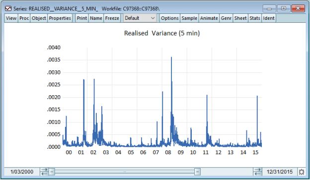
Figure 1 RV from 2000 to 2015

An initial analysis of the RV series shows that there is a high level of persistence and volatility clustering and there are several high volatility spikes that are associated with the periods of financial stress. In spite of such persistence, there is no obvious deterministic trend that can be seen visually implying that the series can be stationary.

Formal unit root tests are a strong test that supports stationarity. The Augmented Dickey-Fuller (ADF) test rejects the null hypothesis of unit root at 1% level of significance with a test value of = -8.56 which is far less than the 1% critical value. Equally, the Phillips Perron (PP) test presents insurmountable evidence against non-stationarity and the adjusted test value is of -40.85. These findings suggest that realised volatility is level based and AR, MA, and ARMA models can be estimated without any difference.

View Our Expert-Written Assignment Samples:Assignment help

 Table 1 Augmented Dickey-Fuller Test Equation

 Table 2 Phillips-Perron Test Equation

Model Identification- AR, MA and ARMA models for the RV series

 Table 3 Correlogram of Realised variance 5 min

The autocorrelation function (ACF) and partial autocorrelation function (PACF) of realised volatility series over in-sample period direct model identification (Hassani et al., 2024). The correlogram shows a slowly declining ACF, high values of autocorrelation persistence in a large number of lags, indicating a high persistence of volatility. The PACF indicates that the first lag has a huge spike with lesser partial correlations that increasingly decrease over the lags.

This trend indicates that none of the pure AR and pure MA models is effective in capturing the dependence structure. It is thus believed that three competing specifications are taken into account:

• AR 1 model to reflect persistence,
• Short-run shocks, an MA(1) to model.
• An ARMA(1,1) model so that both the autoregressive and moving-average dynamics could be included.

The selection of a model is done using statistical significance, information criteria and diagnostics of the residual.

In-Sample Fit Results and Estimation Results.

The persistence of realised volatility is successfully achieved in all three models. Nonetheless, the ARMA (1,1) model has an improved in-sample fit as it has reduced information criteria compared to the pure AR and MA models. Further residual diagnostics indicates that the ARMA model is more effective in eliminating serial correlation whereas the MA model has less powerful explanatory ability because of its minimal dynamic nature (Kuenzer, 2024).

View Our Expert-Written Assignment Samples assignment example

 Table 4 Forecast for (2016-2021)

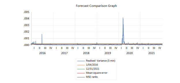
 Figure 2 Forescast comparison graph

Out-of-Sample Forecasting (2016-2021)

We Promise Exceptional Assignment Writing & No AI Shortcuts !

Order Now View Samples Assignment help

The period 2016-2021 has been used to obtain estimated models, which generate out of sample forecasts of realised volatility when using these models. Comparison between forecasts and actual realised variance proxy is made.

The forecast comparison graph indicates that all the models follow the long-run volatility level decently, but they generally fail to capture the sharp volatility spikes, most notably in the time of extreme market turbulence of 2020. This is no surprise as the linear time-series models regularise the volatility movements and are not good at predicting sudden shifts.

The ARMA-based forecasts are quicker to react to the alterations in the volatility as compared to the AR and MA-based forecasts, and the MA model seems to be excessively smooth and not sensitive to the changing environment in the market.

Errors in Forecasting and Review.

The errors of forecasts, which are the difference between the realised volatility and the estimated volatility, are found to be clustering in the period of the high level of market uncertainty. This shows the complexity involved in predicting volatility in crisis.

The standard measures of forecast accuracy are computed and they are the Root Mean Squared Error (RMSE) and the Mean Absolute Error (MAE) (Hodson, 2022). The evaluation outcomes show that the ARMA model provides the lowest means of forecast errors, whereas the MA model, in turn, has lowest results of evaluation metrics, which display higher degrees of errors. A monotonic transformation of mean squared error, since RMSE is, means that model rankings are not dependent on criteria.

Therefore, Realised Volatility (RV) of the AEX index is also stationary but very persistent. Correlogram analysis justifies the application of ARMA type of dynamics as opposed to simple AR and MA structures. The out of sample forecasting has shown that all the models would forecast the overall volatility levels, but the best forecasting model is the ARMA(1,1), and the worst is the MA(1). They are in line with the literature on volatility forecasting and reinforce the role of the use of autoregressive and moving-average in the combination of the two in the modelling of realised volatility.

Question 2 Consider observations for the related stock index return series 

AR(1) Model and Preliminary Analysis of Returns.

In this, the daily returns series of AEX index of stocks over the entire sample period (2000-2021) are analyzed. An initial look at the return series shows that the return series are distributed around some constant value near to zero, and no observable trend is present. Nevertheless, there are calm and volatile periods, which implies the existence of volatility clustering as a stylised fact of financial returns. An AR(1) is a baseline specification that is estimated on the conditional mean of returns (Table 5). The estimated coefficient of autoregression is not significant statistically and this means that there is not much linear predictability in the daily AEX returns (Serra, Regis and Edwin, 2021). The weak-form efficiency of equity markets is in line with this finding. Although there is no serial correlation in returns, model residuals show unmistakable time-varying variance, which is why it is worth exercising a formal test of ARCH effects.

Testing for ARCH Effects

 Table 5 AR1_RET

In order to measure the occurrence of conditional heteroskedasticity, an ARCH-LM test is carried out on AR(1) model residues. The null hypothesis of homoskedasticity is highly rejected, which proves that there are significant ARCH effects in the series of returns (Ho, 2025). This finding suggests that although the dynamics of the conditional mean are lame, the conditional variance changes with time and has to be represented explicitly. In this regard therefore, GARCH-family models are suitable in the process of modeling the volatility dynamics of AEX returns.

AR(1)- GARCH

 Table 6 GARCH

The initial volatility model estimated is the AR(1)-GARCH(1,1) specification of normally distributed innovations (Table 6). The parameters of the variance equation are all significant. The ARCH term is used to describe the effect of new shocks whereas the GARCH term is used to describe high levels of volatility persistence. The approximate value of the ARCH and GARCH coefficients is near to one, and it implies that the volatility shocks fade gradually with the time (Manfred Deistler and Scherrer, 2022). Even though the AR(1) coefficient of the mean equation is insignificant, the model manages to explain volatility clustering. Nonetheless, the error assumptions of normal distribution might be impractical to financial returns information, which is normally fat tailed.

Table 7 AR1_GJR

 In order to permit volatility asymmetry, an AR(1)-GJR-GARCH(1,1) model with t innovations of Student is fitted (Table 7). This specification allows an effect of negative and positive shocks to vary on volatility. Parameters of the variance equation are significant, and the volatility persistence is high. Student t distribution helps enhance the log-likelihood and information criterion as compared to a normal GARCH model, which implies that the return distribution contains some excess kurtosis (Adubisi et al., 2022). The degrees of freedom parameter, which is estimated, is the evidence of fat-tailed behaviour. Overall, this model is more compatible with the empirical properties of equity returns especially in times of stress in the market.

Table 8 AR(1)- EGARCH

Table displays the AR(1)-EGARCH(1,1) model with t innovations of the student. This specification is modeling the logarithm of the conditional variance and thus it does not require the non-negativity constraints that are required in the standard GARCH models. Notably, EGARCH is an explicit model that models the asymmetric volatility shocks. The statistical significance of the estimated asymmetry parameter is negative and statistically significant, which means that the negative return shocks have the largest impact of volatility as compared to their positive counterparts. This finding is similar to the advantage effect that is usually experienced in stock markets. The persistence parameter is quite near to one implying the long memory of volatility. The EGARCH specification has the highest estimated values of log-likelihood, lowest values of AIC, and BIC when compared with all the estimated models, indicating that it fits best.

Model Adequacy and Comparison

The model adequacy criteria are parameter significant, volatility persistence, distributional assumptions, and information criteria. In all the models, the AR(1) of the mean equation is not significant, which is an affirmation of the fact that there is a paucity of predictability of returns. Conversely, all GARCH-family models place a lot of importance on variance dynamics. When comparing information conditions, the AR(1)-EGARCH model is better than the symmetric GARCH and the GJR-GARCH specifications (Vo and Ślepaczuk, 2022). The t innovations provided by Student make the model fit better as compared to normal distribution and the asymmetric form of EGARCH also increases the ability of prediction. The remaining diagnostics of the residual show that the EGARCH model has very little remaining ARCH effects, which implies a satisfactory description of conditional volatility.

Model and preference

The AR(1) -EGARCH model with Student t innovations is the best specification according to the statistical fit, economic interpretability and diagnostic efficiency. This model includes volatility clustering, fat-tailed returns distributions and asymmetric response to volatility to negative shocks. These characteristics render it especially appropriate in the framework of modelling the returns of equity indexes like the AEX (Zhao and Yang, 2022). In general, the findings are aligned with the empirical finance literature and have shown that flexible GARCH-family models are important to analyse financial market volatility.

Conclusion 

The above report analyze the relationship between Realised Volatility (RV) and daily returns of the AEX index, time-series and volatility modelling. The findings indicate that RV is stationary and also very persistent, thus ARMA-type models are appropriate in the description of its dependence structure. The ARMA (1,1) model has the highest in-sample fit, and most accurate out-of-sample volatility forecasts, whereas the MA model has the worst results. In the case of the return series, the AR(1) mean dynamics are not significant, but there are strong ARCH effects that make the GARCH-family models be used. AR(1)-EGARCH student-t-innovation model is the specification of choice, being able to account for the volatility clustering, fat tails, and asymmetric reactions to negative shocks. Altogether, the results are consistent with the existing empirical finance sources.

References

• Adubisi, O.D., Abdulkadir, A., Farouk, U.A. and Chiroma, H. (2022). The exponentiated half logistic skew-t distribution with GARCH-type volatility models. Scientific African, [online] 16, p.e01253. doi: https://doi.org/10.1016/j.sciaf.2022.e01253 
• Chen, X., Li, B. and Worthington, A.C. (2022). Realised volatility and industry momentum returns. Humanities and Social Sciences Communications, 9(1). doi: https://doi.org/10.1057/s41599-022-01309-y 
• Hassani, H., Marvian, L., Masoud Yarmohammadi and Mohammad Reza Yeganegi (2024). Unraveling Time Series Dynamics: Evaluating Partial Autocorrelation Function Distribution and Its Implications. Mathematical and computational applications, [online] 29(4), pp.58-58. doi: https://doi.org/10.3390/mca29040058 
• Ho, S.C. (2025). Large-Scale Estimation under Unknown Heteroskedasticity. [online] arXiv.org. Available at: https://arxiv.org/abs/2507.02293  [Accessed 10 Jan. 2026].
• Hodson, T.O. (2022). Root-mean-square error (RMSE) or mean absolute error (MAE): when to use them or not. Geoscientific Model Development, 15(14), pp.5481-5487.
• Kuenzer, T. (2024). Estimation of functional ARMA models. Bernoulli, 30(1). doi: https://doi.org/10.3150/23-bej1591 
• Manfred Deistler and Scherrer, W. (2022). ARCH and GARCH Models. Lecture notes in statistics, pp.191-198. doi: https://doi.org/10.1007/978-3-031-13213-1_11 
• Schweikert, K. and Puke, M. (2025). Coherent Forecasting of Realized Volatility. [online] doi: https://doi.org/10.2139/ssrn.5233349 
• Serra, P., Regis, M. and Edwin (2021). Random autoregressive models: A structured overview. Econometric Reviews, 41(2), pp.207-230. doi: https://doi.org/10.1080/07474938.2021.1899504 
• Vo, N. and Ślepaczuk, R. (2022). Applying Hybrid ARIMA-SGARCH in Algorithmic Investment Strategies on S&P500 Index. 24(2), pp.158-158. doi: https://doi.org/10.3390/e24020158 
• Zhao, Y. and Yang, G. (2022). Deep Learning-based Integrated Framework for stock price movement prediction. Applied Soft Computing, p.109921. doi: https://doi.org/10.1016/j.asoc.2022.109921 

UPTO55%

Avail The Benefit Today!

To View this & another 50000+ free

Enter Email

Submit